データ型

データ型#

from helper.python import print_subclasses
from helper.jupyter import row
import numpy as np
import polars as pl

Polars は、データを効率よく管理・操作するために、さまざまなデータ型を用意しています。この章では、Polars で利用できるデータ型を詳しく紹介し、それぞれの特徴と用途を説明します。数値型、時系列型、ネスト型などがどのように構造化され、データ処理でどのように役立つかを理解すれば、Polars の機能を十分に活かせます。

データ型の継承木#

Polars のデータ型は多様で柔軟です。次の継承木は、各データ型がどのように構造化されているかを示し、特性や用途を理解する助けになります。NumericType や TemporalType のような主要な型はさらに細かい型に分かれ、それぞれ特定の処理に最適化されています。NestedType は複雑なデータ構造を支え、Boolean や String といった基本型も幅広い処理を可能にします。

print_subclasses(pl.DataType)

└──DataType
   ├──NumericType
   │  ├──IntegerType
   │  │  ├──SignedIntegerType
   │  │  │  ├──Int8
   │  │  │  ├──Int16
   │  │  │  ├──Int32
   │  │  │  ├──Int64
   │  │  │  └──Int128
   │  │  └──UnsignedIntegerType
   │  │     ├──UInt8
   │  │     ├──UInt16
   │  │     ├──UInt32
   │  │     ├──UInt64
   │  │     └──UInt128
   │  ├──FloatType
   │  │  ├──Float16
   │  │  ├──Float32
   │  │  └──Float64
   │  └──Decimal
   ├──TemporalType
   │  ├──Date
   │  ├──Time
   │  ├──Datetime
   │  └──Duration
   ├──NestedType
   │  ├──List
   │  ├──Map
   │  ├──Array
   │  └──Struct
   ├──ObjectType
   │  └──Object
   ├──Boolean
   ├──String
   ├──Binary
   ├──Categorical
   ├──Enum
   ├──Null
   ├──Unknown
   └──BaseExtension
      └──Extension

数値型

NumericType: 数値型の基底クラス。整数型や浮動小数点型などの数値データを扱います。
- IntegerType: 整数データを表すクラスの基底クラス。
  - SignedIntegerType: 符号付き整数データ（Int8、Int16、Int32、Int64）
  - UnsignedIntegerType: 符号なし整数データ（UInt8、UInt16、UInt32、UInt64）
- FloatType: 浮動小数点データを表すクラスの基底クラス（Float32、Float64）
- Decimal: 固定小数点数データを扱います。高精度の数値計算に使用されます。

時系列型

TemporalType: 時間に関連するデータ型の基底クラス。
- Date: 日付データを扱います（例: 2024-07-18）。
- Time: 時刻データを扱います（例: 12:34:56）。
- Datetime: 日時データを扱います（例: 2024-07-18 12:34:56）。
- Duration: 時間の期間を扱います（例: 5分、2時間）。

ネスト型

NestedType: ネスト構造を持つデータ型の基底クラス。
- List: 要素のリストを扱います。リスト内の要素は同じデータ型でなければなりません。
- Array: 固定長の配列を扱います。
- Struct: 構造体データを扱います。異なるデータ型を持つ複数のフィールドを持てます。

その他のデータ型

Boolean: 真偽値データを扱います（True または False）。
String: 文字列データを扱います。
Binary: バイナリデータを扱います。
Categorical: カテゴリカルデータを扱います。効率的にカテゴリ値を管理します。
Enum: 列挙型データを扱います。
Object: 任意の Python オブジェクトを扱います。特定のデータ型に適合しないデータを格納するために使用されます。
Null: NULL 値を扱います。欠損値を示すために使用されます。
Unknown: 未知のデータ型を扱います。

データ型変換#

Cast#

Polars には、データ型の変換に使う関数がいくつかあります。ここでは cast() と shrink_dtype() の2つを取り上げます。

df = pl.DataFrame(
    {
        "a": [3, 3, 3, 4],
        "b": [4, 12, 6, 7],
        "g": ['B', 'A', 'A', 'C']
    }
)
df

shape: (4, 3)

a	b	g
i64	i64	str
3	4	"B"
3	12	"A"
3	6	"A"
4	7	"C"

cast() は、列を指定したデータ型に変換します。整数型を浮動小数点型にしたり、文字列型を日付型にしたりと、データの表現を変えたいときに使います。

df.with_columns(
    pl.col.a.cast(pl.UInt8),
    pl.col.b.cast(pl.String)
)

shape: (4, 3)

a	b	g
u8	str	str
3	"4"	"B"
3	"12"	"A"
3	"6"	"A"
4	"7"	"C"

shrink_dtype() は、値の範囲に合わせてデータ型を必要最小限のサイズに縮めます。たとえば Int64 の列が実際には Int8 で足りるなら、メモリを 1/8 にできます。

Polars 2.0 では式（Expr）からは呼べなくなり、Series のメソッドになりました。列ごとに適用して、新しいデータフレームを作ります。

df2 = pl.DataFrame({name: df[name].shrink_dtype() for name in df.columns})

print(df.dtypes)
print(df2.dtypes)

[Int64, Int64, String]
[Int8, Int8, String]

8ビットや16ビットの整数で、符号付きと符号なしの間で変換する場合は、cast() の wrap_numerical 引数を True にします。

df = pl.DataFrame(
    [
        pl.Series("A", [1, 2, -1, -2], dtype=pl.Int16),
        pl.Series("B", [1, 2, 0xffff, 0xfffe], dtype=pl.UInt16)
    ]
)

df.select(
    pl.col('A').cast(pl.UInt16, wrap_numerical=True),
    pl.col('B').cast(pl.Int16, wrap_numerical=True),
)

shape: (4, 2)

A	B
u16	i16
1	1
2	2
65535	-1
65534	-2

データ型再定義#

cast() が数値を変換するのに対し、NumPy の .view() のように、バイト表現はそのままで別の型として解釈したい場合があります。そのようなときは reinterpret() を使います。

Polars の最新バージョンでは、Expr.reinterpret() に dtype を指定すると、符号付き/符号なし整数の変換だけでなく、同じバイトサイズの任意の数値型に再解釈できます。

次の例では、誤って UInt64 として保存されたデータを Float64 として解釈し直します。

df_wrong = pl.DataFrame({"nums": [4837362400224322580, None, 4837362400224322584]}, schema={"nums": pl.UInt64})
df_fixed = df_wrong.select(pl.col("nums").reinterpret(dtype=pl.Float64))
row(df_wrong, df_fixed)

shape: (3, 1)

nums
u64
4837362400224322580
null
4837362400224322584

shape: (3, 1)

nums
f64
2.5000e15
null
2.5000e15

reinterpret() の signed 引数を使うと、符号付き整数と符号なし整数の間で解釈し直せます。signed=False で符号なし、signed=True で符号付きになります。

reinterpret(dtype=...) を使えば、整数と浮動小数点数の相互変換もできます。ただし、変換元と変換先のデータ型は同じバイトサイズでなければなりません。たとえば Int32 から Int64 への再解釈は、サイズが異なるためエラーになります。

次のコードでは、signed 引数を使った符号付き/符号なし整数の変換を示します。

df = pl.DataFrame(
    [
        pl.Series("A", [1, 2, -1, -2], dtype=pl.Int32),
        pl.Series("B", [1, 2, 0xffffffff, 0xfffffffe], dtype=pl.UInt32)
    ]
)

df.with_columns(
    pl.col('A').reinterpret(signed=False),
    pl.col('B').reinterpret(signed=True)
)

shape: (4, 2)

A	B
u32	i32
1	1
2	2
4294967295	-1
4294967294	-2

バイナリ文字列から同じバイト数のデータ型に変換するには、bin.reinterpret() を使います。dtype で変換後のデータ型、endianness でバイトオーダー（"big" または "little"）を指定できます。次の例では、バイナリデータを4バイトの符号なし整数（UInt32）として、ビッグエンディアンで解釈します。

df = pl.DataFrame({
    'binary_column': [b'\x00\x00\x00\x01', b'\x00\x00\x00\x02', b'\x00\x00\x00\x03', b'\x00\x00@A']
})

df.select(pl.col('binary_column').bin.reinterpret(dtype=pl.UInt32, endianness="big"))

shape: (4, 1)

binary_column
u32
1
2
3
16449

次に、reinterpret() の実用例として、『Quake III Arena』の C 言語のソースコードにある高速逆平方根（Fast inverse square root）の計算を見てみましょう。このコードは、魔法の数字 0x5f3759df を使って浮動小数点数を整数として解釈し直すことで、平方根の逆数を効率よく計算しています。

float Q_rsqrt( float number )
{
 long i;
 float x2, y;
 const float threehalfs = 1.5F;

 x2 = number * 0.5F;
 y = number;
 i = * ( long * ) &y; // 浮動小数点数のビットレベルハック
 i = 0x5f3759df - ( i >> 1 ); // 魔法の数字
 y = * ( float * ) &i;
 y = y * ( threehalfs - ( x2 * y * y ) ); // 最初のニュートン反復
 return y;
}

Polars の reinterpret(dtype=...) を使えば、NumPy の .view() と同様のビットレベルハックを Polars のエクスプレッション API 内で実現できます。以下、NumPy での実装と Polars での実装を比較します。

import numpy as np
number = np.linspace(0.1, 10, 100)
y = number.astype(np.float32)  #❶
x2 = y * 0.5
i = y.view(np.int32)  #❷
i[:] = 0x5F3759DF - (i >> 1)  #❸
y = y * (1.5 - x2 * y * y)  #❹
np.max(np.abs(1 / np.sqrt(number) - y))  #❺

np.float64(0.005045614041059743)

同じ計算を Polars の reinterpret() で実装します。cast() は数値を変換しますが、reinterpret() はバイト表現をそのままにして型だけを変更する点がポイントです。

❶ NumPy の astype() に相当し、cast(pl.Float32) で値そのものを変換します。

❷ NumPy の .view(np.int32) に相当し、reinterpret(dtype=pl.Int32) で浮動小数点数のバイト列を整数として再解釈します。

❸ 整数として再解釈した値に対して // 2（右シフト相当）を計算し、魔法の数字 0x5F3759DF を引きます。その後、reinterpret(dtype=pl.Float32) で結果を再び浮動小数点数に戻します。Polars の表現チェーン内で完結している点が NumPy 版とは異なります。

❹ ニュートン反復で、平方根の逆数の近似値を計算します。

❺ 真の値と近似値の間の最大誤差を表示します。

import polars as pl
import numpy as np

# PolarsのreinterpretでQ_rsqrtを実装
number = np.linspace(0.1, 10, 100)
df = pl.DataFrame({"number": number})

result = (
    df.with_columns(pl.col("number").cast(pl.Float32).alias("y"))  #❶
    .with_columns((pl.col("y") * 0.5).alias("x2"))
    .with_columns(pl.col("y").reinterpret(dtype=pl.Int32).alias("i"))  #❷
    .with_columns(
        (0x5F3759DF - pl.col("i") // 2)  #❸
        .reinterpret(dtype=pl.Float32)
        .alias("y_approx")
    )
    .with_columns(
        (pl.col("y_approx") * (1.5 - pl.col("x2") * pl.col("y_approx") * pl.col("y_approx")))
        .alias("y_result")  #❹
    )
)

y_result = result["y_result"].to_numpy()
max_err = np.max(np.abs(1.0 / np.sqrt(number) - y_result))
print(f"最大誤差: {max_err}")  #❺
result.head(5)  # 結果の一部を表示

最大誤差: 0.005045614041059743

shape: (5, 6)

number	y	x2	i	y_approx	y_result
f64	f32	f32	i32	f32	f32
0.1	0.1	0.05	1036831949	3.26486	3.157232
0.2	0.2	0.1	1045220557	2.26486	2.23551
0.3	0.3	0.15	1050253722	1.83243	1.825705
0.4	0.4	0.2	1053609165	1.63243	1.578616
0.5	0.5	0.25	1056964608	1.43243	1.41386

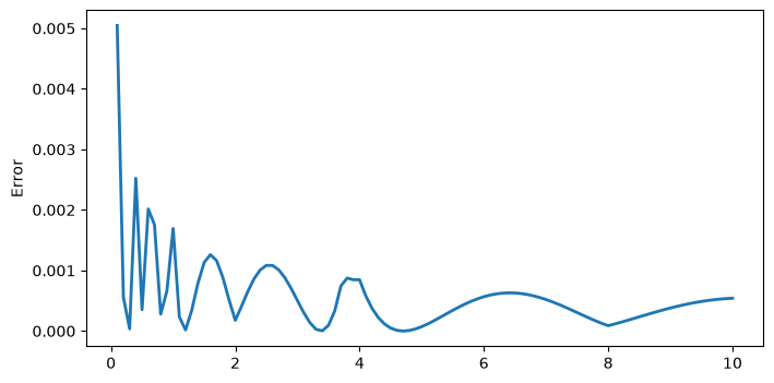
誤差の分布を可視化します。number が小さいときは絶対誤差が大きくなりますが、そのとき関数の値も大きいため、相対誤差の変化はそれほど大きくありません。

import matplotlib.pyplot as plt
y_result = result["y_result"].to_numpy()

plt.figure(figsize=(8, 4))
plt.plot(number, 1 / np.sqrt(number) - y_result, lw=2)
plt.ylabel("Error");

_images/d165beea57248355b32c226cf13967cc3251c177799fbf99738da377d1f06f2b.png

文字列#

Polars は文字列の処理にも強みがあります。文字列を扱う式は .str ネームスペースにまとまっています。

文字列の長さ#

str.len_chars() — 文字数を数えます。マルチバイト文字（日本語など）も1文字として数えます。
str.len_bytes() — バイト数を数えます。マルチバイト文字は複数バイトとして数えられます。

df = pl.DataFrame({
    "lib": ["pandas", "numpy", "polars", "図形"],
    "ver": ["2.0", "1.1.4", "1.2.1", "4.0"]
})

df.select(
    "lib",
    len_char=pl.col("lib").str.len_chars(),
    len_byte=pl.col("lib").str.len_bytes()
)

shape: (4, 3)

lib	len_char	len_byte
str	u32	u32
"pandas"	6	6
"numpy"	5	5
"polars"	6	6
"図形"	2	6

文字列の部分一致検索#

str.contains()、str.starts_with()、str.ends_with() などの関数で、特定の部分文字列が含まれるか、指定された文字列で始まるか、終わるかをチェックできます。既定ではリテラルとして照合し、正規表現として解釈させたいときは literal=False を渡します。ここを取り違えると、意図しない行が大量に一致します。

df.filter(pl.col.lib.str.starts_with("p"))

shape: (2, 2)

lib	ver
str	str
"pandas"	"2.0"
"polars"	"1.2.1"

df.filter(pl.col.ver.str.ends_with("0"))

shape: (2, 2)

lib	ver
str	str
"pandas"	"2.0"
"図形"	"4.0"

df.filter(pl.col.lib.str.contains('p'))

shape: (3, 2)

lib	ver
str	str
"pandas"	"2.0"
"numpy"	"1.1.4"
"polars"	"1.2.1"

.contains() では正規表現を使えます。次のコードは、バージョンに点が2つある行を取り出します。

df.filter(pl.col.ver.str.contains("^\d+\.\d+\.\d+$"))

<>:1: SyntaxWarning: "\d" is an invalid escape sequence. Such sequences will not work in the future. Did you mean "\\d"? A raw string is also an option.
<>:1: SyntaxWarning: "\d" is an invalid escape sequence. Such sequences will not work in the future. Did you mean "\\d"? A raw string is also an option.
C:\Users\ruoyu\AppData\Local\Temp\ipykernel_11752\1031424121.py:1: SyntaxWarning: "\d" is an invalid escape sequence. Such sequences will not work in the future. Did you mean "\\d"? A raw string is also an option.
  df.filter(pl.col.ver.str.contains("^\d+\.\d+\.\d+$"))

shape: (2, 2)

lib	ver
str	str
"numpy"	"1.1.4"
"polars"	"1.2.1"

.str.contains_any() は、文字列やパターンのリストのうち、いずれかが含まれているかを判定します。複数のキーワードを一度に調べたいときに便利です。

df2 = pl.DataFrame({
    "text": ["hello world", "data process library", "data science", "machine learning", "plot library"]
})

df2.filter(
    pl.col("text").str.contains_any(["science", "machine"])
)

shape: (2, 1)

text
str
"data science"
"machine learning"

.str.contains_any() の引数には式も渡せます。列をそのまま渡すと「1つの文字列」と解釈されるので、implode() でリストにしてから渡します。次のコードは、text 列で出現頻度が上位2つの単語を含む行を取り出します。

expr = (
    pl.col.text.str.split(" ").explode().value_counts(sort=True).head(2).struct.field("text")
)
# implode() で「値のリスト」にしてから contains_any に渡す
row(df2.select(expr), df2.filter(pl.col("text").str.contains_any(expr.implode())))

shape: (2, 1)

text
str
"data"
"library"

shape: (3, 1)

text
str
"data process library"
"data science"
"plot library"

文字列の置換#

.str.replace() と .str.replace_all() で、指定した部分文字列を置き換えます。

str.replace() — 最初に見つかった1つの一致だけを置き換えます。
str.replace_all() — すべての一致を置き換えます。

df2.select(pl.col.text.str.replace_all('data', 'DATA'))

shape: (5, 1)

text
str
"hello world"
"DATA process library"
"DATA science"
"machine learning"
"plot library"

文字列の分割#

文字列を特定の区切り文字で分割できます。

df2.with_columns([
    pl.col("text").str.split(" ").alias("split")
])

shape: (5, 2)

text	split
str	list[str]
"hello world"	["hello", "world"]
"data process library"	["data", "process", "library"]
"data science"	["data", "science"]
"machine learning"	["machine", "learning"]
"plot library"	["plot", "library"]

df2.with_columns([
    pl.col("text").str.split_exact(" ", 1).alias("split_exact")
])

shape: (5, 2)

text	split_exact
str	struct[2]
"hello world"	{"hello","world"}
"data process library"	{"data","process"}
"data science"	{"data","science"}
"machine learning"	{"machine","learning"}
"plot library"	{"plot","library"}

文字列のトリミング#

文字列の前後の空白や特定の文字を除去します。

df3 = pl.DataFrame({
    "text": [" hello ", " world", "polars ", "is ", " awesome"]
})

df3.with_columns([
    pl.col("text").str.strip_chars(" ").alias("stripped"),
    pl.col("text").str.strip_prefix(" ").alias("no_prefix"),
    pl.col("text").str.strip_suffix(" ").alias("no_suffix")
    
])

shape: (5, 4)

text	stripped	no_prefix	no_suffix
str	str	str	str
" hello "	"hello"	"hello "	" hello"
" world"	"world"	"world"	" world"
"polars "	"polars"	"polars "	"polars"
"is "	"is"	"is "	"is"
" awesome"	"awesome"	"awesome"	" awesome"

str.strip_chars() — 両端の空白を削除します。
str.strip_prefix() — 指定した接頭辞を先頭から削除します。
str.strip_suffix() — 指定した接尾辞を末尾から削除します。

文字列のパディング#

文字列の左右、または片方に特定の文字で埋めてパディングを行います。

df2.with_columns([
    pl.col("text").str.pad_start(20, "-").alias("padded")
])

shape: (5, 2)

text	padded
str	str
"hello world"	"---------hello world"
"data process library"	"data process library"
"data science"	"--------data science"
"machine learning"	"----machine learning"
"plot library"	"--------plot library"

文字列からパターンに一致した部分を取り出すには、str.extract、str.extract_all、str.extract_groups、str.extract_many などの関数を使います。

str.extract(pattern, group_index) は、正規表現に一致した特定のキャプチャグループを返します。引数は次の2つです。

pattern — 正規表現パターンを指定します。取り出したい部分を () で囲んだキャプチャグループとして書きます。グループは複数作ることもでき、それぞれに 1, 2, 3, … の番号が割り当てられます。
group_index — キャプチャグループの番号を指定します。正規表現の中のどのグループを取り出すかを決めます。

次のコードでは、pattern に2つのキャプチャグループを定義し、group_index で アイテム A と アイテム B の数値を取り出します。

df = pl.DataFrame({
    "text": ["Item A: 50, Item B: 30", "Item A: 70, Item B: 45"]
})

pattern = r'Item A: (\d+), Item B: (\d+)'

df.select(
    pl.col("text").str.extract(pattern, 1).alias("A_value"),
    pl.col("text").str.extract(pattern, 2).alias("B_value"),
)

shape: (2, 2)

A_value	B_value
str	str
"50"	"30"
"70"	"45"

str.extract_groups() は、正規表現のすべてのキャプチャグループを取り出し、構造体（Struct）列として返します。

グループ名を指定しない場合、グループ番号（1, 2, 3, …）がフィールド名になります。

(
df.select(
    pl.col('text').str.extract_groups(pattern).alias('values')
)
.unnest('values')
)

shape: (2, 2)

1	2
str	str
"50"	"30"
"70"	"45"

正規表現内で 名前付きキャプチャグループ (?P<name>...)を使用した場合、その名前がフィールド名になります。

pattern_named = r'Item A: (?P<A_value>\d+), Item B: (?P<B_value>\d+)'

(
df.select(
    pl.col("text").str.extract_groups(pattern_named).alias('values')
)
.unnest('values')
)

shape: (2, 2)

A_value	B_value
str	str
"50"	"30"
"70"	"45"

str.extract_all() は、正規表現に基づいてマッチしたすべての部分をリストとして返します。

df.select(
    pl.col("text").str.extract_all(r'\d+').alias('values')
)

shape: (2, 1)

values
list[str]
["50", "30"]
["70", "45"]

Polars には、re.split() のように正規表現で文字列を分割する関数はありません。代わりに、次のコードでは extract_all() で分割パターンを含む部分をすべて取り出し、list.eval() で各文字列から分割パターンを削除することで、同じ処理を実現しています。

次のコードでは、次の手順で処理します。

extract_all() で、分割パターン（and|after|or|then）を含む部分をすべて取り出します。
list.eval() の中で str.replace() を使い、分割パターンを空文字（""）に置き換えます。

こうすることで、Polars でも re.split() のような文字列分割ができます。

df = pl.DataFrame(
    {"text": [
        "DOGandCATafterFISHorBIRDthenMOUSE",
        "a or b or c"
    ]})

pattern = "and|after|or|then"

def split(expr, pattern):
    return expr.str.extract_all(rf".*?({pattern}|$)").list.eval(pl.element().str.replace(pattern, ''))

df.select(pl.col('text').pipe(split, pattern)).get_column('text').to_list()

[['DOG', 'CAT', 'FISH', 'BIRD', 'MOUSE'], ['a ', ' b ', ' c']]

str.extract_many() は、Aho-Corasick アルゴリズムを使って、文字列から指定したパターンに一致する部分をすべて取り出す関数です。正規表現ではなく、文字列リテラルだけで照合します。大量のデータでも効率よく検索できます。引数は次のとおりです。

patterns — 検索する文字列パターンのリスト。["apple", "banana", "orange"] のように、探したい単語や文字列を並べます。
ascii_case_insensitive — 大文字・小文字を区別しない照合にするかどうか。
overlapping — 重なり合う一致を許すかどうか。True にすると、同じ文字列内で複数のパターンが重なっている場合も、それぞれを別の一致として扱います。

df = pl.DataFrame({
    "text": ["I like apples and bananas", "I prefer oranges and pineapples"]
})

# "apple"と"banana"を検索
df.select(
    pl.col("text").str.extract_many(["apple", "banana"]).alias("matches")
)

shape: (2, 1)

matches
list[str]
["apple", "banana"]
["apple"]

Enum と Categorical#

Enum 型（列挙型）は、決まった値の集合から選ばれるデータ型です。定義した値以外を受け付けないため、データの一貫性を保ち、誤った値の混入を防げます。

Categorical 型（カテゴリカル型）は、有限個のカテゴリーを持つデータ型で、同じ値の重複を避けてメモリ効率を高めます。各カテゴリーに整数のインデックスを割り当てることで、使用メモリを減らします。

Enum はあらかじめ作成し、要素とその順序が固定されています。一方、Categorical は事前の作成が不要で、要素の順序はデータ内の出現順になります。

score = pl.Enum(['A', 'B', 'C', 'D'])
df = pl.DataFrame(
    {
        "a": [3, 3, 3, 4],
        "b": [4, 12, 6, 7],
        "g": ['B', 'A', 'A', 'C']
    }
)
df2 = df.select(
    pl.col.g.cast(score).alias('g_enum'),
    pl.col.g.cast(pl.Categorical).alias('g_cat')
)
df2

shape: (4, 2)

g_enum	g_cat
enum	cat
"B"	"B"
"A"	"A"
"A"	"A"
"C"	"C"

to_physical() を使用すると、内部で保存されている番号を取得できます。次の結果では、g_enum の番号は score で定義された番号であり、g_cat の番号は元の列の値が出現する順番に基づいています。

df2.select(pl.all().to_physical())

shape: (4, 2)

g_enum	g_cat
u8	u32
1	0
0	1
0	1
2	2

次のコードは、Categorical 列で異なるコードを使う場合の違いを示しています。コードの異なる2つの Categorical 列同士で計算すると、処理が遅くなることがあります。

df3 = pl.DataFrame(dict(
    c1 = pl.Series(["Polar", "Panda", "Brown", "Brown", "Polar"], dtype=pl.Categorical),
    c2 = pl.Series(["Panda", "Brown", "Brown", "Polar", "Polar"], dtype=pl.Categorical),
))

df3.with_columns(pl.all().to_physical().name.suffix('_code'))

shape: (5, 4)

c1	c2	c1_code	c2_code
cat	cat	u32	u32
"Polar"	"Panda"	3	4
"Panda"	"Brown"	4	5
"Brown"	"Brown"	5	5
"Brown"	"Polar"	5	3
"Polar"	"Polar"	3	3

次に、pl.StringCache() を使って、同じカテゴリ表を共有する Categorical 列を作ります。

注釈

Polars 2.0 では StringCache は非推奨で、pl.Categories に置き換わる予定です。動作は変わりませんが、実行すると非推奨の警告が出ます。

with pl.StringCache() as s:
    df4 = pl.DataFrame(dict(
        c1 = pl.Series(["Polar", "Panda", "Brown", "Brown", "Polar"], dtype=pl.Categorical),
        c2 = pl.Series(["Panda", "Brown", "Brown", "Polar", "Polar"], dtype=pl.Categorical),
    ))
    
df4.with_columns(pl.all().to_physical().name.suffix('_code'))

C:\Users\ruoyu\AppData\Local\Temp\ipykernel_11752\2951187117.py:1: DeprecationWarning: the string cache has been replaced by pl.Categories
  with pl.StringCache() as s:

shape: (5, 4)

c1	c2	c1_code	c2_code
cat	cat	u32	u32
"Polar"	"Panda"	3	4
"Panda"	"Brown"	4	5
"Brown"	"Brown"	5	5
"Brown"	"Polar"	5	3
"Polar"	"Polar"	3	3

List と Array#

1つの要素に複数の値を保存するには、List 列か Array 列を使います。Array 列は各要素の長さが一定である必要がありますが、List 列は要素ごとに長さが違ってもかまいません。要素を処理する式は、それぞれ array と list ネームスペースにあります。

参考

list 列のメモリレイアウト
 各リスト要素を処理する式

次のコードでは、a_list と b_arr という列を持つ DataFrame を作り、schema でそれぞれのデータ型を pl.List(pl.Int8) と pl.Array(pl.Int8, 3) に定義します。List 列のデータ型は pl.List(element_dtype)、Array 列は pl.Array(element_dtype, length) で定義されます。element_dtype は要素のデータ型、length は各配列の長さです。

df = pl.DataFrame(
    dict(
        a_list=[[1, 2], [3, 4], [5, 6, 7]],
        b_arr=[[1, 2, 3], [3, 4, 5], [5, 6, 7]]
    ),
    schema=dict(a_list=pl.List(pl.Int8), b_arr=pl.Array(pl.Int8, 3))
)
df

shape: (3, 2)

a_list	b_arr
list[i8]	array[i8, 3]
[1, 2]	[1, 2, 3]
[3, 4]	[3, 4, 5]
[5, 6, 7]	[5, 6, 7]

次のコードでは、list ネームスペース内の max()、mean()、len() を使用して、a_list 列の各リストの最大値、平均値、要素数を計算し、新しい列として追加します。また、b_arr 列の各配列の最大値を arr.max() で計算します。arr ネームスペースは比較的新しく、バージョン 1.24.0 では arr.len() と arr.mean() はまだサポートされていません。

df.with_columns(
    a_max=pl.col("a_list").list.max(),
    a_mean=pl.col("a_list").list.mean(),
    a_len=pl.col("a_list").list.len(),
    b_max=pl.col("b_arr").arr.max(),
)

shape: (3, 6)

a_list	b_arr	a_max	a_mean	a_len	b_max
list[i8]	array[i8, 3]	i8	f64	u32	i8
[1, 2]	[1, 2, 3]	2	1.5	2	3
[3, 4]	[3, 4, 5]	4	3.5	2	5
[5, 6, 7]	[5, 6, 7]	7	6.0	3	7

`get` と `gather`#

list.get(index) または arr.get(index) を使うと、指定した index の要素を取り出せます。次のコードでは、a_list 列の各リストの最初の要素と最後の要素の合計を計算します。b_arr 列でも同じ処理をします。

df.with_columns(
    a_first_plus_last = pl.col('a_list').list.get(0) + pl.col('a_list').list.get(-1),
    b_first_plus_last =pl.col('b_arr').arr.get(0) + pl.col('b_arr').arr.get(-1), 
)

shape: (3, 4)

a_list	b_arr	a_first_plus_last	b_first_plus_last
list[i8]	array[i8, 3]	i8	i8
[1, 2]	[1, 2, 3]	3	4
[3, 4]	[3, 4, 5]	7	8
[5, 6, 7]	[5, 6, 7]	12	12

list.gather(indices) を使用すると、複数のインデックスを指定して要素を取得し、新しいリスト列に保存できます。null_on_oob の既定値は False で、範囲外のインデックスを指定するとエラーになります。True にすると、範囲外のインデックスは Null で埋められます。次のコードは、リスト a_list の各要素に対して、インデックス [2, 1, 0] の順に要素を取得し、範囲外のインデックスがある場合は Null で埋める処理を行います。

df.select(
    'a_list',
    gather=pl.col('a_list').list.gather([2, 1, 0], null_on_oob=True)
)

shape: (3, 2)

a_list	gather
list[i8]	list[i8]
[1, 2]	[null, 2, 1]
[3, 4]	[null, 4, 3]
[5, 6, 7]	[7, 6, 5]

`concat_list` と `concat_arr`#

pl.concat_list() は、指定した列や式の結果をリストとして結合し、複数の列の値を1つのリスト列にまとめます。一方、pl.concat_arr() は複数の式の結果を配列として結合します。

df = pl.DataFrame(
    {
        "a": [3, 3, 3, 4],
        "b": [4, 12, 6, 7],
        "g": ['B', 'A', 'A', 'C']
    }
)

df.with_columns(
    pl.concat_list(['a', 'b', pl.col('a') + pl.col('b')]).alias('ab_list'),
    pl.concat_arr(['a', 'b', pl.col('a') + pl.col('b')]).alias('ab_arr'),
)

shape: (4, 5)

a	b	g	ab_list	ab_arr
i64	i64	str	list[i64]	array[i64, 3]
3	4	"B"	[3, 4, 7]	[3, 4, 7]
3	12	"A"	[3, 12, 15]	[3, 12, 15]
3	6	"A"	[3, 6, 9]	[3, 6, 9]
4	7	"C"	[4, 7, 11]	[4, 7, 11]

pl.concat_list() で複数の列を1つのリスト列にまとめたあと、.list の下のメソッドでいろいろな計算ができます。たとえば、次のプログラムでは次の計算を行います。

A、C、E 列の行ごとの総和。行ごとの総和なら pl.sum_horizontal() も使えます。
行ごとの中央値

df_numbers = pl.DataFrame(
    np.random.randint(0, 10, size=(6, 5)), schema=list("ABCDE")
)
df_numbers.with_columns(
    pl.concat_list('A', 'C', 'E').list.sum().alias('sum_ACE'),
    pl.sum_horizontal(pl.col('A', 'C', 'E')).alias('sum_ACE2'),
    pl.concat_list('*').list.median().alias('median_all')
)

shape: (6, 8)

A	B	C	D	E	sum_ACE	sum_ACE2	median_all
i32	i32	i32	i32	i32	i32	i32	f64
4	3	7	3	2	13	13	3.0
8	8	6	5	3	17	17	6.0
8	6	6	3	8	22	22	6.0
5	7	4	0	2	11	11	4.0
4	5	0	9	5	9	9	5.0
3	7	4	4	2	9	9	4.0

reshape#

Expr.reshape() は numpy.reshape() に似ていて、1つの列の要素を指定した数ずつ横に並べる関数です。次の例では、reshape() を使ってデータフレームの列の形状を変更しています。

row(
    df_numbers.select(pl.col('*').reshape((-1, 3))),
    df_numbers.select(pl.col('*').reshape((-1, 2))),
)

shape: (2, 5)

A	B	C	D	E
array[i32, 3]	array[i32, 3]	array[i32, 3]	array[i32, 3]	array[i32, 3]
[4, 8, 8]	[3, 8, 6]	[7, 6, 6]	[3, 5, 3]	[2, 3, 8]
[5, 4, 3]	[7, 5, 7]	[4, 0, 4]	[0, 9, 4]	[2, 5, 2]

shape: (3, 5)

A	B	C	D	E
array[i32, 2]	array[i32, 2]	array[i32, 2]	array[i32, 2]	array[i32, 2]
[4, 8]	[3, 8]	[7, 6]	[3, 5]	[2, 3]
[8, 5]	[6, 7]	[6, 4]	[3, 0]	[8, 2]
[4, 3]	[5, 7]	[0, 4]	[9, 4]	[5, 2]

implode と explode#

Expr.implode() は、式の出力を1つのリスト列に変換します。次のプログラムは、各列の最初の3行のデータをリストにまとめます。

df = pl.DataFrame(dict(A=[1, 2, 3, 4], B=["X", "Y", "X", "Z"]))
df.select(pl.col('*').head(3).implode())

shape: (1, 2)

A	B
list[i64]	list[str]
[1, 2, 3]	["X", "Y", "X"]

Expr.explode() は、リストの要素を縦に展開します。次のプログラムでは、リスト列 value の要素を縦に並べ、group 列の各要素を Expr.repeat_by() で value の各リストの長さだけ繰り返します。

pl.col("group").repeat_by(pl.col("value").list.lengths()) は、group 列の各要素を value 列の各リストの長さ回繰り返します。
pl.col("value").explode() は、value 列のリストを縦に展開します。

結果として、group 列の各要素は対応する value 列の要素に合わせて繰り返されます。

df = pl.DataFrame(dict(group=["B", "A", "A", "C"], value=[[3, 4], [1, 2, 6], [1], [2, 3]]))

df.select(
    pl.col.group.repeat_by(pl.col.value.list.len()).explode(),
    pl.col.value.list.explode()
)

shape: (8, 2)

group	value
str	i64
"B"	3
"B"	4
"A"	1
"A"	2
"A"	6
"A"	1
"C"	2
"C"	3

DataFrame.explode() は Expr.explode() と同じ処理をしますが、他の列のデータを自動的に繰り返します。次のプログラムでは、リスト列 value の要素を縦に並べ、他の列（group 列）のデータを繰り返します。

df.explode('value')

shape: (8, 2)

group	value
str	i64
"B"	3
"B"	4
"A"	1
"A"	2
"A"	6
"A"	1
"C"	2
"C"	3

List 列と Array 列の相互変換#

list.to_array() と arr.to_list() を使うと、List 列と Array 列を相互に変換できます。arr.to_list() はそのまま変換できますが、list.to_array() の場合、要素の長さを引数として渡す必要があり、List 列の要素の長さが一致しない場合はエラーになります。

df = pl.DataFrame(
    dict(
        a=[[1, 2], [3, 4], [5, 6]],
        b=[[1, 2, 3], [3, 4, 5], [5, 6, 7]]
    ),
    schema=dict(a=pl.List(pl.Int8), b=pl.Array(pl.Int8, 3))
)

df.with_columns(
    a_to_arr=pl.col('a').list.to_array(2),
    b_to_list=pl.col('b').arr.to_list()
)

shape: (3, 4)

a	b	a_to_arr	b_to_list
list[i8]	array[i8, 3]	array[i8, 2]	list[i8]
[1, 2]	[1, 2, 3]	[1, 2]	[1, 2, 3]
[3, 4]	[3, 4, 5]	[3, 4]	[3, 4, 5]
[5, 6]	[5, 6, 7]	[5, 6]	[5, 6, 7]

長さがばらばらの List 列を Array 列にするには、list.gather() で足りない位置に NULL を入れて長さをそろえてから変換します。インデックスは implode() でリストにして渡します。

df = pl.DataFrame(
    dict(a=[[1, 2], [3, 4], [5, 6, 7], [8, 9, 10, 11]]),
    schema=dict(a=pl.List(pl.Int8)),
)
df.with_columns(
    a_arr=pl.col("a")
    .list.gather(pl.int_range(end=4).implode(), null_on_oob=True)
    .list.to_array(4)
)

shape: (4, 2)

a	a_arr
list[i8]	array[i8, 4]
[1, 2]	[1, 2, … null]
[3, 4]	[3, 4, … null]
[5, 6, 7]	[5, 6, … null]
[8, 9, … 11]	[8, 9, … 11]

Struct 列への変換#

list.to_struct() は、リスト列の各要素を構造体のフィールドに変換します。フィールド名と個数は fields で指定します。リストが長い場合は、指定した個数を超えた分が落ちます。

df = pl.DataFrame(dict(values=[[1, 2], [2, 3, 4], [1, 10]]))
df2 = df.select(pl.col.values.list.to_struct(fields=["a", "b"]))
row(df, df2)
print(df2.schema)

shape: (3, 1)

values
list[i64]
[1, 2]
[2, 3, 4]
[1, 10]

shape: (3, 1)

values
struct[2]
{1,2}
{2,3}
{1,10}

Schema({'values': Struct({'a': Int64, 'b': Int64})})

リスト列同士の計算#

Polars では、リスト列同士でも、リスト列と数値列の間でも算術演算ができます。

リスト列同士の演算 — 各行で、対応するリストの要素ごとに演算が行われます。
リスト列と数値列の演算 — 数値列の値が各リストの全要素に適用されます。

以下は具体的な例です。このデータフレームでは、x 列と y 列の要素がリストで、各行のリストの長さは一致しています。また、z 列は数値列です。

df = pl.DataFrame(dict(
    x=[[1, 3, 3], [4, 5, 7, 8]], 
    y=[[10, 20, 30], [40, 50, 60, 80]],
    z=[10, 20]    
))

df.with_columns(
    x_plus_y = pl.col('x') + pl.col('y'),
    x_plus_z = pl.col('x') + pl.col('z'),
)

shape: (2, 5)

x	y	z	x_plus_y	x_plus_z
list[i64]	list[i64]	i64	list[i64]	list[i64]
[1, 3, 3]	[10, 20, 30]	10	[11, 23, 33]	[11, 13, 13]
[4, 5, … 8]	[40, 50, … 80]	20	[44, 55, … 88]	[24, 25, … 28]

ビットのリストから整数に変換#

リスト型の列の各要素と、単一のリストの要素を対応させて計算するには、単一のリストを持つ Series を作るか、リストを直接扱う式を使います。以下は、ビットのリストを整数に変換するプログラムで、この計算方法について説明します。

このコードでは、df_bits に格納されたビットのリストを整数値に変換します。ビット列 [b7, b6, ..., b0] を b7 * 2**7 + b6 * 2**6 + ... + b0 * 2**0 のように計算し、対応する整数値を求めます。

❶事前に 2**i のリストを Series に変換し、それを bits の各要素と掛け算した後、.list.sum() で合計を求めます。
❷pl.int_range(7, -1, -1) を使って 2**i の列を生成し、それを implode() で単一のリストを持つ列に変換した後、bits と掛け算して合計を求めます。

df_bits = pl.DataFrame(dict(
    bits=[
        [0, 1, 1, 0, 1, 1, 0, 0],
        [1, 0, 0, 1, 1, 0, 0, 1],
        [1, 1, 1, 1, 1, 1, 1, 1]
    ]
))

df_val1 = df_bits.select(
    value=(pl.col('bits') * pl.Series(values=[[2**i for i in range(7, -1, -1)]])).list.sum() #❶
)

df_val2 = df_bits.select(
    value=(pl.col('bits') * (2 ** pl.int_range(7, -1, -1)).implode()).list.sum() #❷
)
with pl.Config() as conf:
    conf.set_fmt_table_cell_list_len(10)
    row(df_bits, df_val1, df_val2)

shape: (3, 1)

bits
list[i64]
[0, 1, 1, 0, 1, 1, 0, 0]
[1, 0, 0, 1, 1, 0, 0, 1]
[1, 1, 1, 1, 1, 1, 1, 1]

shape: (3, 1)

value
i64
108
153
255

shape: (3, 1)

value
i64
108
153
255

次のように、各ビットのリストの長さが異なる場合は、int_ranges() で各リストの長さに応じた指数のリストを作り、ビット列を整数に変換します。

pl.col('bits').list.len() - 1: 各リストの長さを取得し、最上位ビットの指数を決定します。
pl.int_ranges(..., -1, -1): 各リストの長さに対応する 2**i の指数部分のリストを作成します。
.list.eval(2 ** pl.element()): 各要素を 2**i に変換します。

df_bits = pl.DataFrame(dict(
    bits=[
        [0, 1, 1, 0, 1, 1, 0, 0],
        [1, 0, 0, 1, 1, 0, 0],
        [1, 1, 1, 1]
    ]
))

df_val = df_bits.select(
    (
        (
            pl.col('bits') * 
            pl.int_ranges(pl.col('bits').list.len() - 1, -1, -1).list.eval(2 ** pl.element())
        )
    ).list.sum()
)
with pl.Config() as conf:
    conf.set_fmt_table_cell_list_len(10)
    row(df_bits, df_val)

shape: (3, 1)

bits
list[i64]
[0, 1, 1, 0, 1, 1, 0, 0]
[1, 0, 0, 1, 1, 0, 0]
[1, 1, 1, 1]

shape: (3, 1)

bits
i64
108
76
15

サポートされていない演算#

Polars 1.24.0 の時点では、リスト列間の演算として算術演算（加算、減算、乗算、除算など）はサポートされていますが、それ以外の演算（例: 比較演算や論理演算）はサポートされていません。そのため、次のコードはエラーになります。

%%capture_except
df.select(
    pl.col('x') * 10 > pl.col('y')
)

InvalidOperationError: cannot perform '>' comparison between series 'x' of dtype: list[i64] and series 'y' of dtype: list[i64]

This error occurred in the following expression:
	[([(col("x")) * (10)]) > (col("y"))]

次の方法を使えば、リスト列の要素同士の計算が可能です。

with_row_index() — 各行にユニークなインデックスを追加します。このインデックスは後でグループ化に使用されます。
explode('x', 'y') — x 列と y 列のリストを展開し、各リストの要素を縦に並べます。これにより、リスト要素の対応が維持されます。
group_by('index') — 行ごとの演算結果を元の形に戻すため、インデックス列でデータをグループ化します。
agg() — 各グループ内で演算します。ここでは、x 列の要素を10倍し、y 列の対応する要素と比較します。
drop('index') — 最後にインデックス列を削除します。

(
df
.with_row_index()
.explode('x', 'y')
.group_by('index')
.agg(
    pl.col('x') * 10 > pl.col('y')
)
.drop('index')
)

shape: (2, 1)

x
list[bool]
[false, true, false]
[false, false, … false]

本書の helper.polars モジュールをインポートすると、DataFrame クラスに list_eval() メソッドが追加されます。リスト列を含むデータフレームに対して、要素ごとの演算を簡潔に書くためのラッパーです。

import helper.polars

df.list_eval(
    (pl.col('x') * 10 > pl.col('y')).alias('flag')
)

shape: (2, 1)

flag
list[bool]
[false, true, false]
[false, false, … false]

Polars の構造体列は、複数のフィールドを持つ複合データ型で、型の異なるデータを1つの列にまとめて格納できます。データを整理し、より複雑な構造を表したいときに役立ちます。データフレームを作るときは、Python の辞書のリストを構造体列に変換できます。

df = pl.DataFrame({
    "person": [
        {"name": "John", "age": 30, "car": "ABC"},
        {"name": "Alice", "age": 65, "car": "VOX"},
        {"name": "Tom", "age": 25, "car": "ABC"},
        {"name": "Bob", "age": 45, "car": "KTL"},
        {"name": "Fun", "age": 18, "car": None},
    ],
    "num": [1, 2, 3, 4, 5],
})

df

shape: (5, 2)

person	num
struct[3]	i64
{"John",30,"ABC"}	1
{"Alice",65,"VOX"}	2
{"Tom",25,"ABC"}	3
{"Bob",45,"KTL"}	4
{"Fun",18,null}	5

フィールドと列の変換#

構造体列を処理する関数は struct ネームスペースにあります。たとえば .struct.field() を使うと、構造体から複数のフィールドを個別の列として取り出せます。

df2 = df.select(
    pl.col('person').struct.field('name', 'age')
)

df2

shape: (5, 2)

name	age
str	i64
"John"	30
"Alice"	65
"Tom"	25
"Bob"	45
"Fun"	18

.struct.field() の逆の操作が pl.struct() です。複数の列を構造体列にまとめられます。次のコードでは、name と age の2つの列を構造体としてまとめ、person という名前の構造体列を作成しています。

df2.select(
    pl.struct('name', 'age').alias('person')
)

shape: (5, 1)

person
struct[2]
{"John",30}
{"Alice",65}
{"Tom",25}
{"Bob",45}
{"Fun",18}

フィールドの演算式#

.struct.with_fields() メソッドを使うと、構造体列に対してフィールドの追加や変換ができます。式の中では、pl.col() の代わりに pl.field() を使ってフィールドを指定します。これにより、構造体の中の特定のフィールドを操作できます。

次の例では、person 列の name を大文字にした name_upper フィールドを追加し、car の null を "Mazda" に置き換えます。また、age と num 列の値を足して、age フィールドを更新します。

df2 = df.select(
    pl.col("person").struct.with_fields(
        pl.field("name").str.to_uppercase().alias('name_upper'),
        pl.field("car").fill_null("Mazda"),
        pl.field("age") + pl.col("num")
    )
)
df2

shape: (5, 1)

person
struct[4]
{"John",31,"ABC","JOHN"}
{"Alice",67,"VOX","ALICE"}
{"Tom",28,"ABC","TOM"}
{"Bob",49,"KTL","BOB"}
{"Fun",23,"Mazda","FUN"}

DataFrame.unnest() は構造体列を複数の列に展開します。

df2.unnest('person')

shape: (5, 4)

name	age	car	name_upper
str	i64	str	str
"John"	31	"ABC"	"JOHN"
"Alice"	67	"VOX"	"ALICE"
"Tom"	28	"ABC"	"TOM"
"Bob"	49	"KTL"	"BOB"
"Fun"	23	"Mazda"	"FUN"

出力は構造体の演算式#

式の出力が構造体になることもあります。たとえば value_count() です。

df_car_count = df2.select(pl.col("person").struct.field("car").value_counts())
print(df_car_count.schema)
df_car_count

Schema({'car': Struct({'car': String, 'count': UInt32})})

shape: (4, 1)

car
struct[2]
{"Mazda",1}
{"ABC",2}
{"VOX",1}
{"KTL",1}

List または Array 列への変換#

次の方法で、構造体列を List 列または Array 列に変換できます。

まず、struct.field('*') を使って全フィールドを選択するか、フィールド名のリストを指定して一部のフィールドを選択します。
各フィールドのデータ型が異なる場合は、必要に応じて cast() を使い、もっとも上位のデータ型に変換します。
concat_list() または concat_arr() を使用して、1つの List 列または Array 列に変換します。

df = pl.DataFrame(dict(
    point=[{"x":1.0, "y":2, "z":3}, {"x":4.0, "y":5, "z":6}]
))

df2 = df.with_columns(
    point_list=pl.concat_list(pl.col('point').struct.field('*').cast(pl.Float64)),
    point_list_2d=pl.concat_list(pl.col('point').struct.field('x', 'y').cast(pl.Float64)),
    point_arr=pl.concat_arr(pl.col('point').struct.field('*').cast(pl.Float64)),
)
df2

shape: (2, 4)

point	point_list	point_list_2d	point_arr
struct[3]	list[f64]	list[f64]	array[f64, 3]
{1.0,2,3}	[1.0, 2.0, 3.0]	[1.0, 2.0]	[1.0, 2.0, 3.0]
{4.0,5,6}	[4.0, 5.0, 6.0]	[4.0, 5.0]	[4.0, 5.0, 6.0]

複数の列を一緒に処理#

複数の列をまとめて処理するには、構造体を使うと便利です。たとえば、次のコードでは A と B 列の値が同じ行のうち、最初の行だけを残します。

df = pl.DataFrame(
    dict(
        A = [1, 2, 1, 2, 1, 2],
        B = [2, 4, 2, 5, 2, 4],
        C = [1, 2, 3, 4, 5, 6]
    )
)

df.filter(
    pl.struct('A', 'B').is_first_distinct()
)

shape: (3, 3)

A	B	C
i64	i64	i64
1	2	1
2	4	2
2	5	4

上のコードは、DataFrame.unique() と同じ結果になります。

df.unique(['A', 'B'], maintain_order=True, keep='first')

shape: (3, 3)

A	B	C
i64	i64	i64
1	2	1
2	4	2
2	5	4

pl.when().then().otherwise() で同じ条件から複数の式を計算するときは、構造体を使うとコードを短くできます。

次のコードでは、A 列の値に応じて B と C 列の値を操作します。

A 列の値が 1 の場合は、B 列に 10、C 列に 100 を加算します。
A 列の値が 1 でない場合は、B 列から 10、C 列から 100 を減算します。

pl.struct() で複数の式を1つの構造体にまとめ、最後に .struct.field() で構造体のフィールドを列に戻します。

df.with_columns(
    pl.when(pl.col('A') == 1)
    .then(
        pl.struct(
            pl.col('B') + 10, 
            pl.col('C') + 100
        )
    )
    .otherwise(
         pl.struct(
             pl.col('B') - 10, 
             pl.col('C') - 100
         )   
    )
    .struct.field('B', 'C')
)

shape: (6, 3)

A	B	C
i64	i64	i64
1	12	101
2	-6	-98
1	12	103
2	-5	-96
1	12	105
2	-6	-94

A	B	C	D	E	sum_ACE	sum_ACE2	median_all
i32	i32	i32	i32	i32	i32	i32	f64
4	3	7	3	2	13	13	3.0
8	8	6	5	3	17	17	6.0
8	6	6	3	8	22	22	6.0
5	7	4	0	2	11	11	4.0
4	5	0	9	5	9	9	5.0
3	7	4	4	2	9	9	4.0

A	B	C	D	E	sum_ACE	sum_ACE2	median_all
i32	i32	i32	i32	i32	i32	i32	f64
4	3	7	3	2	13	13	3.0
8	8	6	5	3	17	17	6.0
8	6	6	3	8	22	22	6.0
5	7	4	0	2	11	11	4.0
4	5	0	9	5	9	9	5.0
3	7	4	4	2	9	9	4.0

データ型

目次

データ型#

データ型の継承木#

データ型変換#

Cast#

データ型再定義#

文字列#

文字列の長さ#

文字列の部分一致検索#

文字列の置換#

文字列の分割#

文字列のトリミング#

文字列のパディング#

Enum と Categorical#

List と Array#

get と gather#

concat_list と concat_arr#

reshape#

implode と explode#

List 列と Array 列の相互変換#

Struct 列への変換#

リスト列同士の計算#

ビットのリストから整数に変換#

サポートされていない演算#

フィールドと列の変換#

フィールドの演算式#

出力は構造体の演算式#

List または Array 列への変換#

複数の列を一緒に処理#

`get` と `gather`#

`concat_list` と `concat_arr`#

A	B	C	D	E	sum_ACE	sum_ACE2	median_all
i32	i32	i32	i32	i32	i32	i32	f64
4	3	7	3	2	13	13	3.0
8	8	6	5	3	17	17	6.0
8	6	6	3	8	22	22	6.0
5	7	4	0	2	11	11	4.0
4	5	0	9	5	9	9	5.0
3	7	4	4	2	9	9	4.0